Oxford Economics Thematic Report July 2026

Oxford Economics, a key adviser to corporate, financial and government decision-makers and thought leaders, prepared this report specifically for Hargreaves Lansdown.
Foreword
People retiring with defined contribution pensions face several complex decisions. After having spent decades building up a pension, they need to decide how best to draw an income and deal with the tricky balancing act of maintaining the standard of living they enjoyed while working and also ensuring that they don’t run out of money.
Retirement income decisions play a major part in this, with all options coming with their own pros and cons.
Although conservative pension drawdown strategies - such as the 4% rule – are designed to limit the risk that households will run out of money in retirement while also giving flexibility, they can result in lower levels of consumption in retirement. This can mean households struggling to maintain their desired standard of living. More aggressive drawdown strategies will allow for higher levels of consumption but increase the risk that households will run out of savings in their later years.
On the other hand, annuities provide an alternative in that they pay out an income for life. However, they reduce financial flexibility and come with a further set of decisions related to the value of annuitised income, the timing of annuity purchase, and whether to protect against inflation.
This report developed in partnership with Oxford Economics explores the extent to which households across the nation are on track to achieve their expected level of spending in retirement—based on their income, age, tenure, and relationship status—under different financial strategies.
Key findings from this analysis are:
Household spending falls gradually across retirement, and this matters for annuity planning. For a high earning household aged 75 to 87, average annual expected spending in retirement is 5.3% lower than for a similar household aged 67–74. The fall is smaller for low-earning households, at just 2.1%. This reflects that their spending is more concentrated on essentials, and therefore there is less scope to cut back as they age. As expected, spending declines only modestly in real terms over retirement and inflation means it is unlikely to fall in nominal terms. As a result, a non-inflation-linked annuity covering expected spending needs at the start of retirement risks being unable to cover expected spending needs later on.
(See Figure 3 below.)
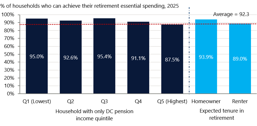
Around 9-in-10 households can cover their expected essential spending by combining the State Pension with an inflation‑linked annuity purchased using their pension pot. According to the analysis, almost all low earners (95%) are able to cover their expected essential spending through this approach, as it is largely covered by the State Pension. This figure falls to 87% for high earners, as a smaller proportion of their expected essential spending is covered by the State Pension.
Under a conservative drawdown strategy (4% pa with the amount increasing by inflation every year), only 56% of households are on track to cover their expected total spending. This compares with 70% under a more aggressive drawdown strategy. However, the aggressive strategy risks households exhausting their pension savings later in life and being left to rely solely on the State Pension, exposing them to a drop in living standards.
Purchasing an inflation linked annuity at 67 allows 61% of households to cover their expected total spending. This strategy protects against the risk of running out of money in later life, and a pooling of risk allows for a 5-percentage-point increase in affordability relative to the conservative drawdown strategy.
Hybrid strategies that combine income drawdown and annuities offer more financial flexibility than an annuity purchased at the start of retirement and allow a larger proportion of households (64%) to achieve their expected spending. The hybrid strategy combines drawdown in early retirement with an inflation-linked annuity later in life. However, this approach increases the risk that assets are depleted too quickly, leaving households unable to purchase the annuity they require later in retirement.
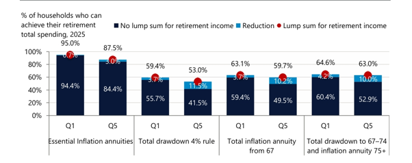
What you do with your tax-free cash matters. Tax-free cash is often used to fund large one-off expenses such as paying off a mortgage or home renovations rather than as part of a retirement income strategy. However, this analysis shows that this can have a real impact on people’s ability to achieve their desired retirement income. The proportion of households on track to cover their expected total spending in retirement falls by around 8 percentage points when the lump sum is not used to provide a retirement income. The impact is bigger for higher earners - around 10 percentage points - as they rely more on their pension wealth and less on the State Pension to support their spending.
(See Figure 12 below.)
The findings highlight the variety of decisions that face people when it comes to managing income throughout their retirement. There are lots of different factors that need to be weighed up and in the case of annuities they can’t be unwound if the wrong one is purchased. Although a lot of emphasis is placed on the importance of building up your pension, this analysis also shows the huge impact these income decisions can also have on your quality of life as you age. Those who take financial advice will find this support invaluable in helping them navigate these challenges. For those who don’t have an adviser, Targeted Support can play a huge role in enabling providers to step in and offer vital support in helping people make these important decisions.
Section 1: Introduction
1.1 Retirement Spending and Planning Considerations
Households entering retirement face a complex set of financial decisions that shape their future living standards. At the core of this is a balance between achieving a desired living standard, ensuring that financial resources do not run out in later life, and maintaining financial flexibility.
The risk of running out of money, driven by uncertainty around lifespan and market volatility, can lead individuals to respond by adopting conservative pension drawdown strategies to preserve their assets. While this provides protection against longevity risk, it can also result in lower living standards than necessary. International evidence, particularly from countries with longer experience of flexible defined contribution systems, suggests that many retirees do not fully decumulate their pension wealth and instead prioritise financial security over consumption.
An annuity can protect against running out of money in later life, but it reduces financial flexibility. Individuals considering an annuity must decide not just whether to annuitise, but also how much spending to target, the timing of annuity purchase, and whether to choose inflation protection. These decisions are particularly important because declines in real spending as retirees age tend to fall more slowly than inflation, making the preservation of purchasing power critical.
A key feature of the UK pension system is the ability to withdraw up to 25% of savings as a tax‑free lump sum. While this supports financial flexibility, it also creates another important retirement decision regarding how to use the lump sum. Evidence shows it is often used for one‑off expenditures and gifts to families rather than generating ongoing income. Spending the lump sum, rather than using it to generate a sustained stream of income in retirement, reduces resources available to fund consumption later in life.
Recent work from the Second Pensions Commission highlights the growing importance of these choices. As defined contribution pensions increasingly dominate the pension landscape, individuals are increasingly responsible for managing pension decumulation. The Commission notes that many individuals may lack the engagement or expertise required, raising concerns about both underspending and the risk of depleting assets too quickly.
This report focuses on defined contribution households and how retirement outcomes change based on different financial decisions. It provides valuable insights for households trying to find the correct balance between achieving their desired living standard, ensuring that financial resources do not run out in later life, and maintaining financial flexibility.
Section 2: Spending during retirement
2.1 Modelling overview
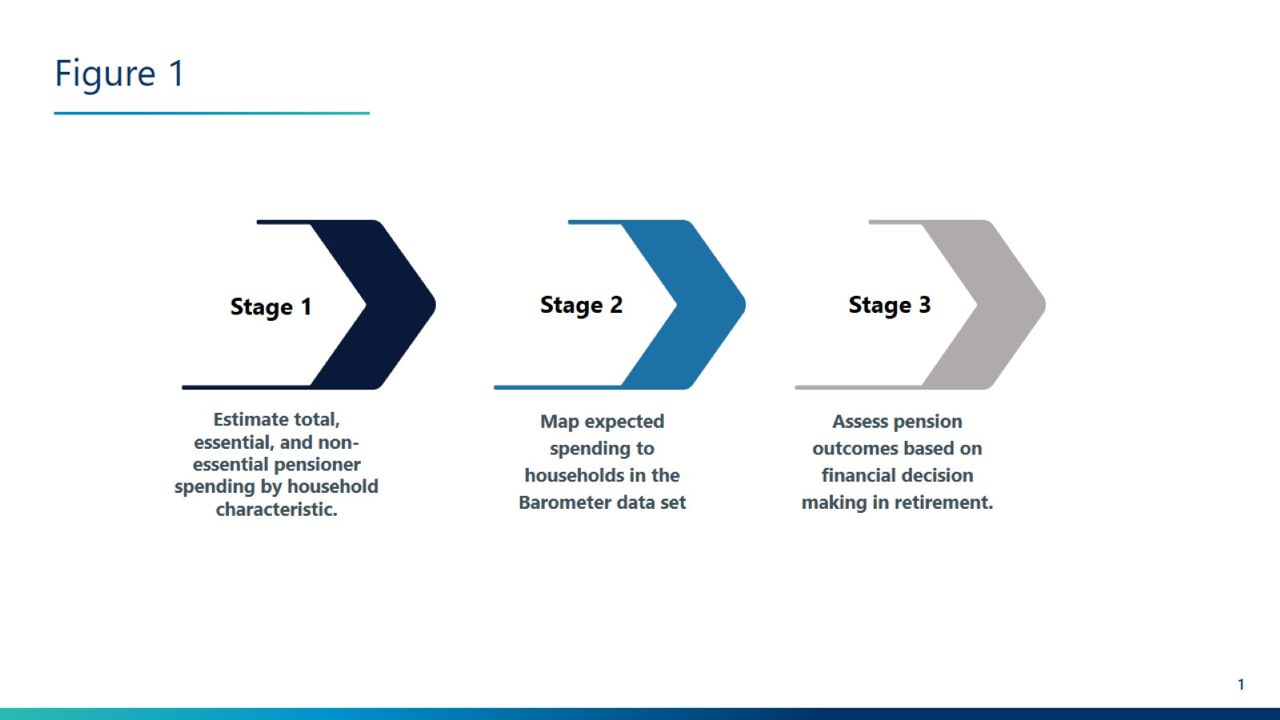
To assess how financial decision‑making influences households’ outcomes in retirement, this report employs a structured three‑stage modelling framework. The analysis draws on the Living Costs and Food Survey (LCFS), which provides detailed information on household expenditure, alongside the Barometer dataset, which contains data on households’ wealth, pension holdings, and demographic characteristics.
In the first stage, retirement spending profiles are estimated for different household types based on combinations of income, age, housing tenure, and relationship status characteristics. These estimates distinguish between total, essential, and non‑essential spending, providing a granular view of how consumption needs in retirement vary across household types. Essential and non‑essential spending are distinguished by separating core living costs from more discretionary expenditure. Essential spending includes items such as housing, utilities, food, transport running costs, and clothing, while non‑essential spending covers items such as leisure activities, holidays, eating out, and home improvements.
In the second stage, these profiles are mapped onto non‑retired households in the Barometer dataset, assigning expected retirement spending based on anticipated retired characteristics, such as retirement tenure and income group. The analysis focuses on households that only have defined contribution (DC) pensions, reflecting their growing importance.
The final stage assesses whether households are on track to meet different retirement outcomes by comparing current pension wealth with projected spending under a range of financial scenarios. These scenarios reflect key decisions, including annuitisation, drawdown behaviour, and use of the tax‑free lump sum. This allows the analysis to capture the central role of decumulation strategies in shaping retirement outcomes.
Two adequacy benchmarks are used in the modelling. The essential spending benchmark assesses whether households can meet core living costs, while the total spending benchmark evaluates whether a household can sustain their current living standard. The model also accounts for how spending evolves over the course of retirement. This enables more realistic projections of income needs and is particularly important for strategies involving delayed annuitisation, where annuity costs are adjusted to reflect lower spending at older ages.
Overall, this framework provides a comprehensive basis for analysing how spending needs, pension wealth, and financial decisions interact to determine retirement outcomes.
2.2 Change in spending during retirement
Understanding how spending evolves through retirement is central to financial planning. Decisions about how pension wealth is converted into income, particularly the timing and structure of annuitisation, depend on expectations about how expenditure will change over time. If spending declines significantly with age, retirees may favour front‑loaded consumption strategies. Conversely, if expenditure remains relatively stable, maintaining real income becomes more important, with implications for inflation protection and longevity risk.
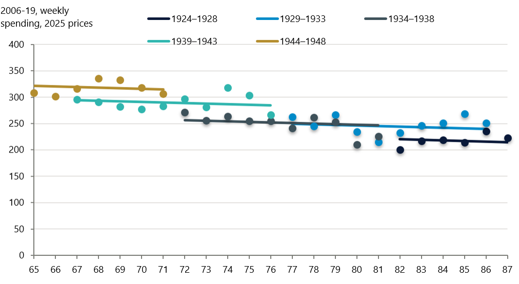
At first glance, cross‑sectional data suggest the median spending falls substantially with age, with snapshot comparisons indicating a decline of around 20% between those aged 65–74 and 75–87. However, this pattern can be misleading as it conflates generational differences with changes within a cohort over time.
Once cohort effects are considered, the decline is much less pronounced, as shown in Figure 2 (below). Analysis tracking spending within cohorts shows only modest reductions. The apparent steep decline largely reflects lower lifetime incomes and wealth among older cohorts. As a result, younger retirees typically spend more, not because spending falls sharply with age, but because they start from a higher baseline.
This distinction has important implications for retirement planning. It suggests large reductions in spending should not be the default planning assumption. Instead, spending is likely to remain relatively stable from year to year and decline gradually over time. Strategies that assume sharp declines may therefore underestimate the income required to sustain living standards later in life.
Figure 2: Total median weekly expenditure by birth cohort and age
2.3 Predicting the retirement spending of households in the barometer
To capture how spending evolves through retirement, expected expenditure is estimated across two age bands: 65–74 and 75–87. This reflects evidence that spending changes gradually over the retirement lifecycle and allows the analysis to distinguish between early and later retirement when assessing income strategies, such as annuitisation, at a later stage in retirement.
Figure 3 (below) shows that spending declines with age across all income groups, though the scale of the decline varies. Higher-income households experience larger spending reductions in both absolute and percentage terms, reflecting their greater share of discretionary spending, which is typically cut back to a greater extent as households age. In contrast, lower-income households see smaller declines, as their spending is more concentrated on essential items, which are more difficult to cut back on. Incorporating essential and total spending into the analysis ensures that financial decisions in retirement are evaluated against multiple retirement living standard benchmarks.
Figure 3: Average retirement spending for ages 67–74 and 75–87 by income quintile
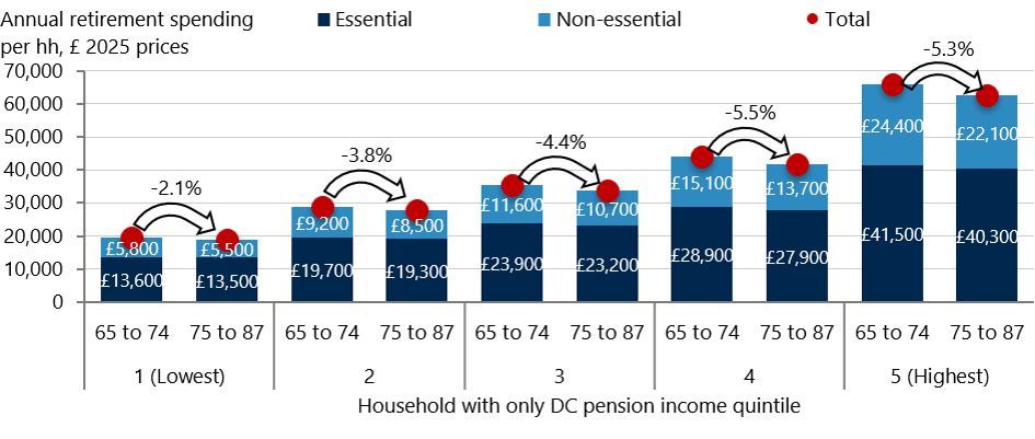
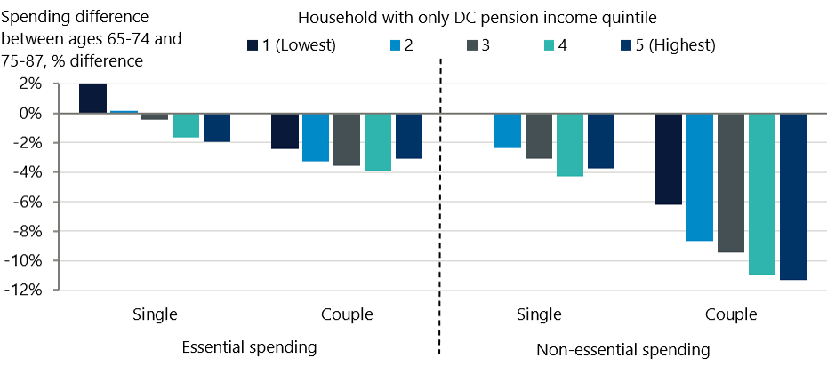
The total household spending estimates in Figure 3 (above) are based on a weighted average of expected spending for single and couple households. However, analysing these groups separately highlights important differences in spending patterns by relationship status over retirement.
As shown in Figure 4 (below), couple households tend to experience larger declines in spending as they age compared with single households. This reflects their ability to adjust expenditure without affecting essential consumption. For couples, many essential costs, such as housing, utilities, and basic living expenses, are shared, reducing the cost per person and creating an inherent saving. This leaves greater scope for discretionary spending, which can be scaled back as they age. In contrast, single individuals face many of these costs on a per‑person basis, leaving less room for discretionary adjustments.
Figure 4: Spending difference between ages 65–74 and 75–87 for singles and couples
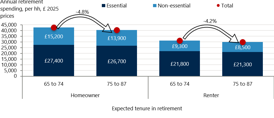
Renters not only spend less overall but also allocate a larger share of their spending to essentials (Figure 5). This reflects the higher housing costs from rental payments, which reduce the scope for discretionary spending and make essential spending a larger proportion of total consumption. Renters tend to experience a smaller overall decline in spending, as a larger share of their expenditure is already concentrated on essential items, leaving less scope to reduce discretionary consumption compared with homeowners.
Figure 5: Average retirement spending for ages 67–74 and 75–87 by expected retirement tenure
Section 3: Pension coverage and withdrawal strategy
3.1 Modelling pension coverage
The ability of households to achieve their expected spending in retirement using their pension pot depends on three key factors: the level of that spending, the financial decisions made when accessing pension wealth, and the size of the household’s accumulated pension pot. Each element plays an important role in determining whether available resources can be converted into a sustainable income that supports desired living standards over the course of retirement.
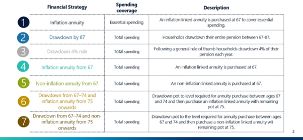
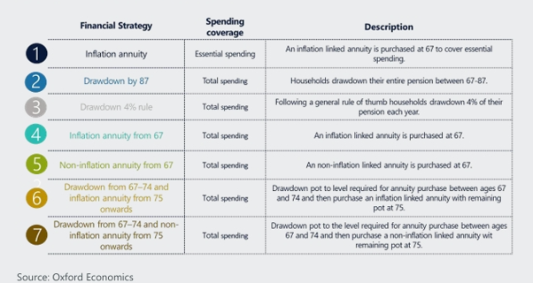
To capture the impact of financial decision‑making, we have modelled seven distinct scenarios that reflect different ways in which households may choose to access and use their pension wealth. These scenarios, set out in Figure 6 (below), are designed to represent a range of plausible strategies, including variations in drawdown behaviour, annuitisation strategies, and consumption benchmarks.
By comparing outcomes across these scenarios, the modelling provides a view of how different retirement strategies perform at a national level in supporting households’ spending needs. This highlights that the ability of households to achieve adequate retirement outcomes varies depending on how pension wealth is used, not just its size.
Figure 6: Financial decision-making scenarios
The modelled scenarios illustrate the key trade‑offs households face when converting pension wealth into retirement income. These centre on balancing income security, flexibility, and affordability, and reflect the increasing complexity of decisions highlighted by the Second Pensions Commission as responsibility has shifted towards individuals.
Income certainty vs. flexibility: Annuities provide a guaranteed income for life, protecting against longevity risk but limiting flexibility. Drawdown approaches offer greater control over withdrawals and spending but create uncertainty for households.
Drawdown strategy and risk of depletion: Strategies that draw down more aggressively support higher consumption but risk leaving households with insufficient income if they live longer than expected. More conservative approaches, such as the 4% rule, reduce this risk, but they can result in lower spending and a higher likelihood of unspent pension wealth.
Inflation protection trade‑off: Inflation‑linked annuities maintain purchasing power and help sustain living standards but require larger pension pots. Non-inflation-linked annuities offer higher initial income at a lower cost, but real income declines over time, potentially reducing later‑life consumption.
Timing of annuitisation: Delaying annuity purchase allows for flexibility and potential investment growth in early retirement, aligning with higher discretionary spending. However, it also increases exposure to market risk, meaning outcomes depend on both investment performance and the timing of annuitisation decisions.
3.2 Pension affordability by withdrawal scenario
The modelling indicates that most households are able to meet their essential spending needs in retirement. As shown in Figure 7, (below) roughly 92% of households can cover essential expenditure by combining the State Pension with income from an inflation‑linked annuity purchased using their defined contribution pension pot. However, excluding the State Pension, this falls to 42%, highlighting its important role as a foundational source of income in retirement, particularly when supplemented by private pension savings.
Coverage varies across the income distribution. Lower‑income households have the highest levels of coverage, with 95% able to meet their essential spending needs through the State Pension and the purchase of an inflation-linked annuity. This largely reflects the fact that the State Pension alone is often sufficient to cover the majority of essential expenditure for these households. In contrast, coverage is lower among higher‑income groups, falling to 87% for the highest quintile. This is driven by their higher expected essential spending in retirement, which requires a higher level of income beyond the State Pension.
Differences are also evident by housing tenure. Renters have lower levels of coverage, at 89%, compared with 94% for homeowners. This gap reflects the additional and ongoing housing costs faced by renters in retirement, which increase their essential spending, making it more difficult to meet this through pension income alone. Homeowners, particularly those without mortgage costs, benefit from lower essential expenditure and therefore achieve higher levels of coverage, emphasising the important role homeownership plays in shaping retirement outcomes.
The results suggest that the current structure of the UK pensions system provides a relatively strong foundation for covering essential spending in retirement. The combination of the State Pension and private savings through automatic enrolment means that most households are on track to meet this benchmark.
Figure 7: Essential spending is largely covered
The remainder of this report focuses on the extent to which households are on track to meet their expected total retirement spending, including both essential and discretionary components, under different financial decision‑making strategies.
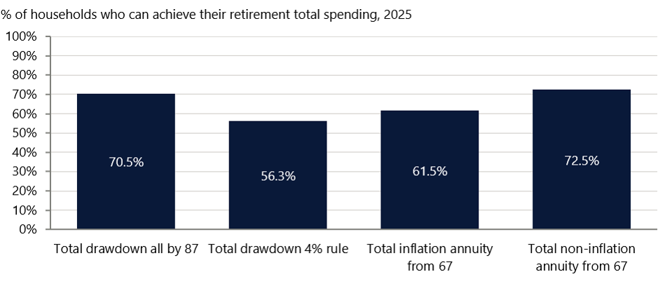
Among the strategies that are maintained throughout the entirety of retirement, the 4% drawdown rule performs worst in terms of affordability. Only around 56% of households are on track to achieve their expected total spending under this approach (Figure 8, below). This reflects the conservative nature of the strategy, which is designed to manage longevity risk at an individual level by limiting withdrawals. While this reduces the probability of running out of money, it also constrains consumption throughout retirement.
In contrast, an inflation‑linked annuity purchased at 67 enables a higher proportion of households to meet their expected spending, with coverage rising to around 62%. This reflects the pooling of longevity risk across individuals, which can allow issuers to provide higher sustainable income compared with self‑managed drawdown strategies. The inflation linkage also helps maintain purchasing power over time, aligning income more closely with spending needs that decline more slowly than prices.
Non‑inflation‑linked annuities appear more affordable at the point of purchase, with around 72% of households able to meet their expected spending initially. However, this comes at the cost of declining real income over time. As shown in Section 2, retirement spending tends to fall more gradually than inflation, meaning that fixed nominal income streams can lead to a deterioration in purchasing power and reduced consumption in later life.
Full withdrawal strategies also perform relatively well in terms of affordability, with around 70% of households able to meet their expected spending. However, this approach carries significant financial risk. By depleting pension wealth more rapidly, households that live beyond the assumed horizon—such as age 87 in this analysis—may be left relying solely on the State Pension, exposing them to a substantial drop in income and living standards in later life.
Figure 8: Differences in affordability across financial strategies
Hybrid strategies, which combine drawdown in early retirement with annuitisation later in life, offer an alternative approach and tend to result in a higher share of households being on track to achieve their expected level of spending in retirement. Drawing down assets in the initial years of retirement allows households to maintain higher levels of spending when discretionary needs are greatest and provides flexibility to respond to changing circumstances. Transitioning to an annuity at older ages then allows households to lock in a stable income stream, helping to reduce longevity risk and ensure a more reliable income in later life.
However, these approaches also introduce additional complexity and risk. They require households to make well‑timed decisions about when to annuitise, which can be difficult given uncertainty around investment performance, life expectancy, and future spending needs. During the drawdown phase, households remain exposed to market and sequencing risk, meaning that adverse returns early in retirement can significantly reduce future income. The Second Pensions Commission highlights that these types of decisions are particularly challenging for individuals and that many may lack the financial capability or engagement to manage them effectively, increasing the likelihood of less favourable outcomes. There is also a risk that assets are depleted too quickly before annuity purchase, leaving insufficient resources to secure an adequate income later in life.
Within hybrid strategies, affordability outcomes are better when non‑inflation‑linked annuities are purchased, with around 69% of households on track to meet their expected spending compared to 64% when inflation‑linked annuities are purchased (Figure 9, below). However, this again reflects the lower upfront cost of non‑inflation annuities and increases the risk of falling purchasing power and reduced living standards in later retirement.
Figure 9: Differences in affordability under hybrid strategies
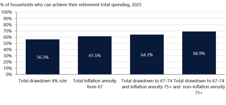
Given the challenges associated with non‑inflation‑linked annuities and full drawdown approaches, these strategies are excluded from the subsequent analysis. While they may appear more affordable in the short term, they entail significant risks to long‑term retirement outcomes.
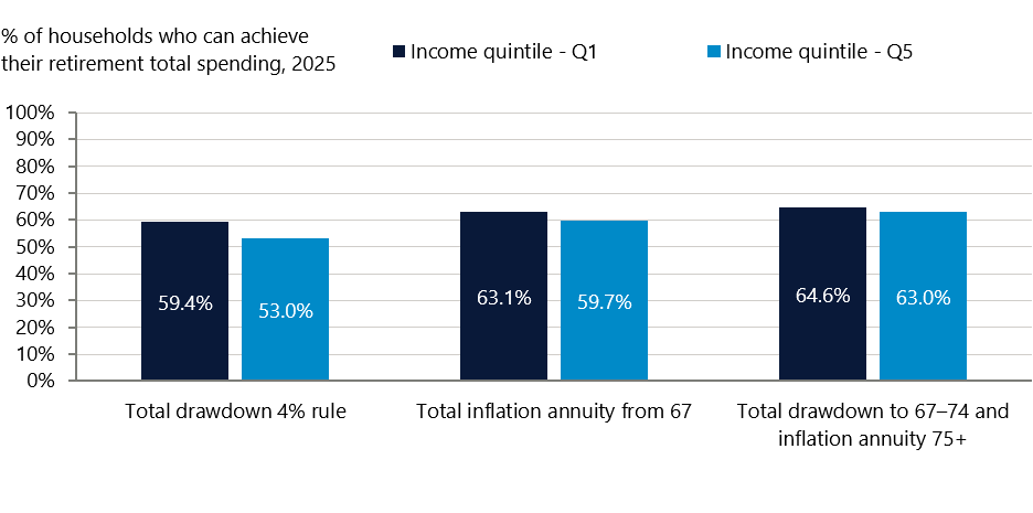
As with the essential spending-based benchmark, the ability to achieve total expected expenditure in retirement varies by income group. Figure 10 (below) shows that lower‑income households are more likely to meet resilience thresholds, largely because the State Pension covers a significant share of their essential spending. Higher‑income households face larger shortfalls, as their expected expenditure is higher and a greater proportion of their income must be generated from defined contribution pension wealth. This dynamic is particularly pronounced under more conservative drawdown strategies, such as the 4% rule, which increases the level of pension wealth required to sustain spending in order to manage longevity risk.
Figure 10: Affordability differences across withdrawal by income group
Section 4: Lump sum uses
4.1 Impact of tax-free lump sum
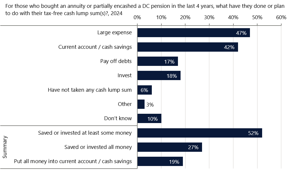
Individuals can access up to 25% of their pension savings as a tax‑free lump sum from retirement age. While this provides a valuable source of flexibility at the point of retirement, evidence suggests that many households do not retain these funds to support ongoing retirement income. Instead, the lump sum is often used for a range of immediate purposes, which reduce the resources available to sustain spending over the longer term.
Common uses for the tax‑free lump sum include large one‑off expenditures such as home improvements, car purchases, and special occasions, as well as transfers to family members. A portion is also sometimes held in cash savings or used to repay outstanding debts. While these uses may improve short‑term financial wellbeing, they are not typically structured to generate a sustained income stream. As a result, this behaviour can create a gap between the level of income implied by total pension wealth and the income that is actually realised in retirement.
The Second Pensions Commission highlights that this pattern is widespread and reflects the broader risks associated with pension decumulation under the current system. High levels of early access to pension wealth, including lump‑sum withdrawals, mean that individuals may draw down resources too quickly or use them inefficiently. Combined with limited guidance and the complexity of retirement decisions, this increases the risk that households enter later retirement with insufficient income, reinforcing the need for stronger support and clearer guardrails around how pension savings are accessed and used.
Figure 11: Use of tax-free lump sum
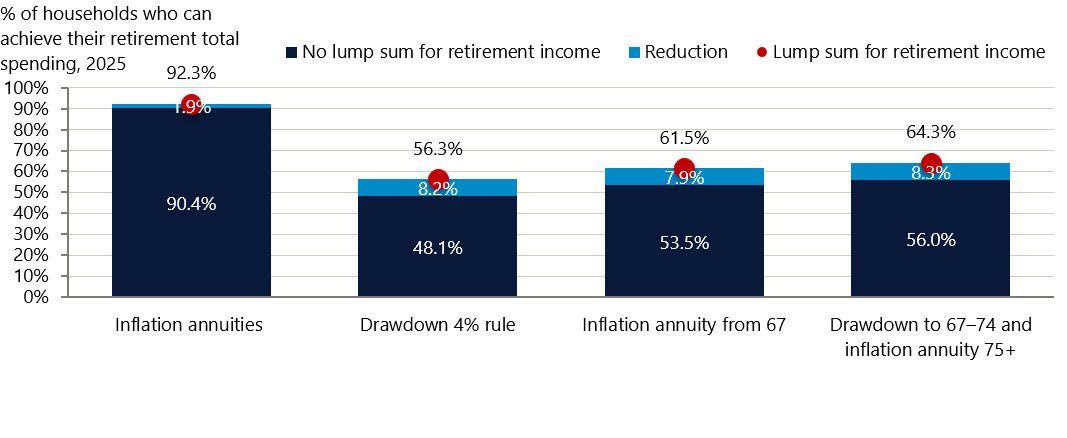
Excluding the tax‑free lump sum from retirement income has a materially different impact depending on the measure of adequacy considered. For essential spending, the effect is relatively limited, reflecting the role of the State Pension in enabling many households to meet their basic needs.
However, the impact becomes significantly more pronounced when total spending is considered. Across the different retirement strategies, the proportion of households able to afford the required pension pot falls by around 8 percentage points when the lump sum is excluded from retirement income. This underscores how decisions about the lump sum taken at retirement shape households’ living standards.
Figure 12: Impact on the proportion of households that can afford the required pension pot if the lump sum is spent on one-off expenses
Excluding the tax‑free lump sum from retirement income has a disproportionate impact across the income distribution. Higher‑income households experience a larger reduction in affordability, as they rely more heavily on defined contribution pension wealth to support both essential and discretionary spending. Removing the lump sum therefore significantly reduces their available resources and increases the likelihood of shortfalls relative to expected consumption. In contrast, lower‑income households are less affected by the exclusion of the lump sum. This reflects the role of the State Pension as a stable income floor, which covers a substantial share of their essential spending and reduces their dependence on private pension wealth.
Figure 13: The reduction of the proportion of households that can afford the required pension pot is largest for higher-income households
Section 5: Methodology appendix
5.1 Overview
This document outlines the methodology used to construct the Hargreaves Lansdown Retirement Expenditure Model, which estimates annual spending for retired households based on a range of demographic and financial characteristics. This document provides details of the data used, modelling steps, assumptions, and outputs underpinning the model. The modelling draws on the Living Costs and Food Survey (LCFS) dataset, which provides empirical spending patterns across birth cohorts of retired households, and the Wealth and Assets Survey (WAS), which is used to assess the proportion of households that can afford the predicted retirement spending based on their pension wealth.
5.2 Dataset and expenditure categorisation
The first step in the methodology is the construction of two expenditure categories—essential and non essential—shown in Figure 14 (below). Classification of Individual Consumption According to Purpose (COICOP) expenditure codes are grouped into six broad spending groupings to support this classification: food and household items; housing and utilities; transport and travel; leisure and lifestyle; healthcare and insurance; and other expenses. Within these groupings, individual expenditure items are classified as either essential or non essential to distinguish core day-to-day spending from more discretionary consumption. The essential expenditure classification is underpinned by an Australian Bureau of Statistics study of discretionary and non discretionary inflation. Total household consumption is defined as the sum of all included essential and non essential expenditure components.
Figure 14: Expenditure categories
| Category | Essential spending | Non-essential spending |
|---|---|---|
| Food and household items | Food, tea, coffee, and items for routine household maintenance | Sugary food, fruit juice, alcohol, tobacco, and other household goods and services |
| Housing and utilities | Housing (including rent and mortgage payments) and utilities | Capital expenditure on homes (home alterations) |
| Transport and travel | Car maintenance, fuel, and insurance | Purchase of vehicles |
| Leisure and lifestyle | Communication, public transport, subscriptions, and pet food | Restaurants, recreation and culture, hotels, and travel insurance |
| Healthcare and insurance | Health expenses and other insurance | – |
| Other expenses | Clothing, footwear, personal care, and debts | Accessories, dry cleaning, and other miscellaneous goods and services |
The analytical sample consists of retired households aged between 65 and 87 drawn from the LCFS, belonging to birth cohorts born between 1924 and 1948. Following the approach adopted in IFS analysis, individuals are grouped into five‑year birth cohorts to facilitate lifecycle comparisons. Retirement status is identified using LCFS labour-market variables, with survey weights applied throughout to maintain representativeness. As the publicly available LCFS data are top‑coded at age 80, we estimate the age distribution for households above this threshold using observed patterns in vehicle ownership, holiday expenditure, and spending on domestic services, alongside relationship status factors associated with ageing. In addition, the proportion of households in each age band is aligned with population distributions from the 2011 and 2021 Census. All estimates are based on the age of the household reference person, reflecting the assumption that spending decisions within couples are made jointly.
To ensure cohort profiles are based on sufficient longitudinal coverage, only age and birth-cohort combinations observed in at least five distinct survey years are retained. The sample is restricted to survey years prior to 2020 to avoid distortions in household spending patterns associated with the Covid-19 pandemic.
5.3 Modelling approach
The model used to generate the expenditure of a retired household by characteristics is built in two stages. First, total median expenditure is estimated using a 50th-percentile quantile regression, creating the central spending anchor for different household types across birth cohorts and age bands. Second, the model determines how this total is split between essential and non-essential spending by estimating budget shares based on the same characteristics. Predicted values are then applied to a population of current working-age households from the WAS.
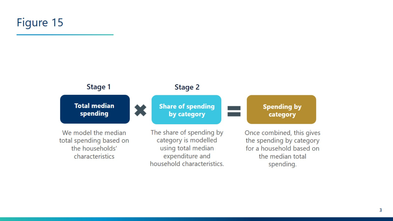
5.3.1 Stage 1: Total expenditure
The first stage models the total median expenditure using a 50th‑percentile quantile regression, with total spending expressed as a function of income, household composition, birth cohort, age band, income decile within cohort and composition group, tenure, and a set of demeaned survey-year indicators to control for year-specific effects. The median is used instead of the mean because it provides a more representative picture of typical spending and remains stable when expenditure patterns are skewed. This is a standard approach for this type of analysis and makes it a more reliable anchor for assessing the spending needs of retired households.
An interaction between age band, income decile within cohort, and household composition is included to capture how spending profiles evolve across the two stages of retirement across these groups. Consistent with the IFS analysis, birth cohort fixed effects and survey-year indicators following the Deaton and Paxson (1994) method are included.
5.3.2 Stage 2: Share of expenditure by category
The second stage allocates total spending between essential and non-essential consumption using a standard Engel curve-based budget share model, a widely used approach in applied consumption analysis. Separate share equations are estimated for essential and non-essential spending using the same demographic and economic characteristics as the total spending equation, with the logarithm of total consumption included to capture how the proportions change as households spend more. This structure reflects well-established Engel curve behaviour where essential items such as Food and household items decline as a share of the budget as total spending rises, while more discretionary areas such as Leisure and lifestyle and Other expenses account for a growing proportion of expenditure.
5.4 Predicting the retirement spending of households in the barometer
Once the two modelling stages are complete, predicted expenditure values are generated for a population of current working-age households in the WAS. Retired tenure and relationship status are modelled first, followed by retirement income.
Retirement tenure: Since retirement tenure is unknown, this has been modelled based on future expected homeownership and the probability of purchasing a home for each renting household. Current homeowners are assumed to remain homeowners in retirement. The expected future homeownership rates are based on Resolution Foundation projections, which estimate that 65% of those currently aged 25, 66% of those aged 35, and 74% of those aged 45 will be homeowners by State Pension age. For renters, the probability of purchasing before retirement is estimated using a logit model with log household income, parental tenure, and education level as predictors. The proportion of homeownership is aligned with these proportions within the respective age groups. Individual households are identified as being homeowners in retirement and are used when generating retirement spending predictions.
Retirement relationship status: As the relationship status of a household at retirement is not known, an average spend for an individual has been calculated based on a weighted average of the single and couple spending. The weighting used has been estimated based on the proportion of individuals who are single or in a couple for the age cohort 65–69. These data show there is a higher proportion of households that are living in a couple compared with being alone. Furthermore, there is a slightly higher probability of an individual being alone if they are currently single. This is due to some individuals not currently living in a couple in this age cohort and having never been in a couple, which does not apply to an individual who is currently in a couple.
Cohort effect: The cohort-specific effect has been set to the cohorts born between 1944–48. Evidence suggests similar spending patterns across adjacent cohorts at overlapping ages, supporting the use of this cohort as a representative baseline.
Retirement income: Retirement income is modelled in two stages. Firstly, retirement income is modelled using a relative ranking approach. In the WAS data, households are assigned to income deciles within detailed age groups and relationship status (single vs. couple), based on total household income. These deciles are assumed to be broadly preserved into retirement, meaning households are mapped to the equivalent position in the retirement income distribution. Second, lifecycle income profiles are estimated using LCFS data for retired households, focusing on the cohort born between 1944–48, consistent with the cohort effect. Because this cohort is not observed across the full retirement period, average income for early (ages 65–74) and later retirement (ages 75–87) is estimated. This is calculated based on historical trends in income between these two periods, controlling for cohort and year effects in a manner consistent with the spending model.
Predicted total consumption, essential spending, and non-essential spending are generated separately for each household under two retirement-age scenarios—early retirement (ages 65–74) and later retirement (ages 75 87)—and under both single- and couple-household assumptions. To align with 2025 consumption patterns, the predicted series has been scaled using macroeconomic consumption trends
5.5 Scenario analysis
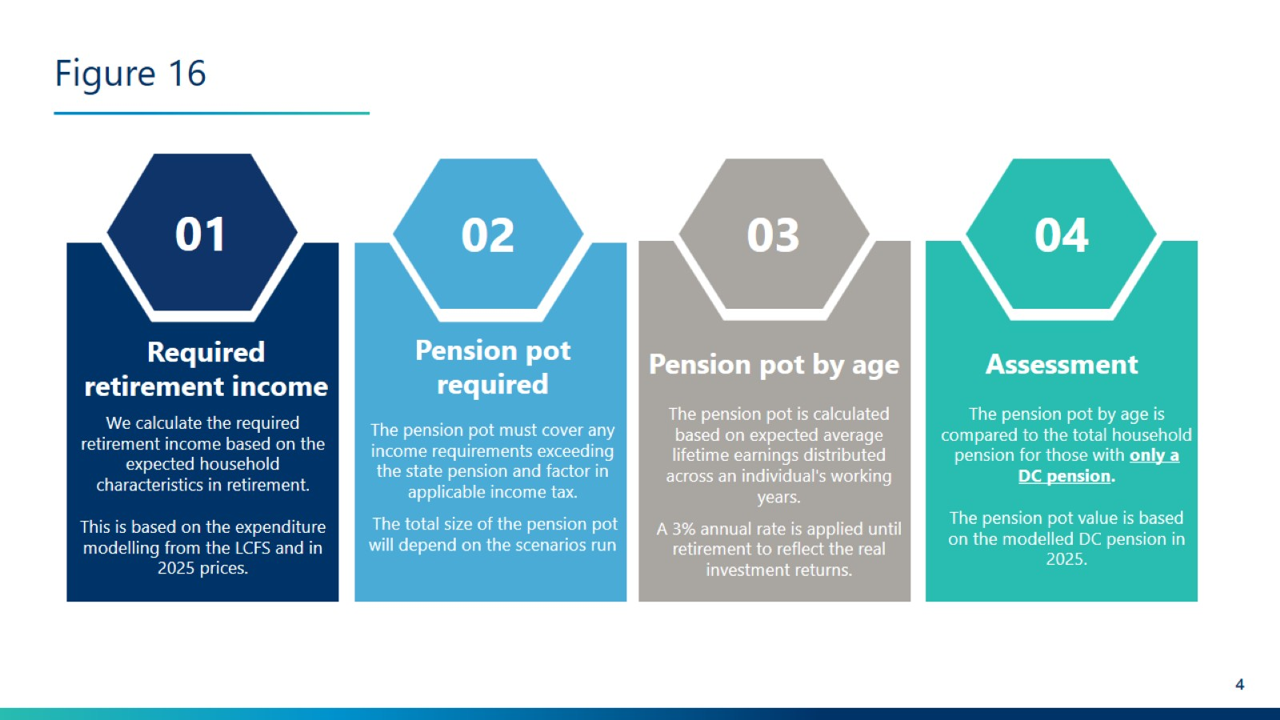
5.5.1 Household pension pot
In addition to the income to support the retirees' spending, households will also need to cover any income tax that must be paid. Individuals currently get £12,570 tax free allowance, so an individual will need to pay tax on the income needed above this threshold. In Section 3, we assume households use the tax-free pension lump sum withdrawal. Therefore, 25% of their pension is tax-free and used to supplement their income during their retirement, and the rest is subject to a 20% tax rate.
These costs will need to be met by the State Pension and pension savings. It is assumed that the State Pension is available to all individuals and equals £230.25 per week. Individuals will need to cover the remaining expenses with pension savings, and the total pension pot required is estimated under each decumulation scenario.
To evaluate how well households are doing in terms of their current pension savings, the total pension pot required has been distributed over the working life of the individuals within the household, enabling comparison with observed DC wealth at a given age. Where households are assumed to take the 25% tax-free lump sum at retirement and spend it on a one-off expense as discussed in Section 4, the required pot is scaled up accordingly to reflect the reduced pot available to generate retirement income.
5.5.2 Scenario assumptions
Seven decumulation scenarios are modelled, varying by financial strategy and spending coverage, as summarised in Figure 17. These scenarios span the main strategies available to households at retirement— annuitisation, drawdown, and hybrid approaches—and are designed to reflect a range of real-world retirement behaviour.
Figure 17: Financial decision-making scenarios
The annuity‑based scenarios use the most recent best‑buy rates, assuming purchases at ages 67 and 75. A weighted average of single‑life and joint‑life (50% survivor benefit) annuities is applied, with weights aligned to the distribution of household types at retirement. The joint‑life annuity is included to reflect the provision of continued income to a surviving partner, ensuring that part of the income stream is maintained in the event of death. For Scenarios 3 and 4, the annuity purchase assumptions are based on the income required in the early years of retirement, rather than an average across the two age groups modelled. This ensures that income is sufficient to meet spending needs during the higher‑spending phase of retirement.
The annuity pricing is summarised in the table below.
Figure 18: Annual income from a £100,000 pension used to buy an annuity

Two pure drawdown scenarios are modelled against total expected spending. The full drawdown scenario assumes households draw down their entire pension pot evenly between ages 67 and 87, with required spending calculated as a weighted average of early retirement (42%) and late-retirement (58%) expenditure— reflecting the share of years spent in each phase of a 21-year retirement. The required pot is calculated using a present value formula assuming a nominal investment return of 5% and real asset growth of 2%. The 4% rule scenario instead assumes households withdraw 4% of their pension pot annually throughout retirement.
Two hybrid scenarios combine drawdown and annuitisation. In both cases, households draw down pension wealth between ages 67 and 74 before purchasing an annuity at age 75 using the remaining pot. The annuity income at age 75 is based on an average of early and later‑retirement spending needs, ensuring that income remains sufficient through the initial years of later retirement. The annuity pot required is then discounted back to age 67 at a rate of 3% per annum, reflecting assumed real growth in the pension assets used to fund the annuity purchase.
For each scenario, a consistent set of estimates is produced under the assumption that the 25% tax-free lump sum is withdrawn at retirement and used for one-off expenditure, leaving a reduced pot to fund ongoing retirement income. This allows the impact of lump-sum withdrawal behaviour on retirement affordability to be quantified.
Text sources
Australian Treasury, Retirement Income Review, November 2020, accessed May 2026
Employee Benefit Research Institute, “Asset Decumulation or Asset Preservation? What Guides Retirement Spending?”, accessed May 2026
Financial Conduct Authority, Financial Lives 2024 survey, accessed May 2026
The Second Pensions Commission, Pensions 2050: Evidence and future priorities – Interim Report, 2026, accessed May 2026.
Australian Bureau of Statistics, Non-Discretionary and Discretionary Inflation, 2020, released May 2026
Institute for Fiscal Studies, “How does spending change through retirement?”, 2022, accessed May 2026
Resolution Foundation, Perfectly adequate?, 2024, accessed May 2026
Figure sources
| Figure 2 | LCFS, Oxford Economics |
| Figure 3 | Oxford Economics |
| Figure 4 | Oxford Economics |
| Figure 5 | Oxford Economics |
| Figure 6 | Oxford Economics |
| Figure 7 | Oxford Economics |
| Figure 8 | Oxford Economics |
| Figure 9 | Oxford Economics |
| Figure 10 | Oxford Economics |
| Figure 11 | Financial Lives Survey, Oxford Economics |
| Figure 12 | Oxford Economics |
| Figure 13 | Oxford Economics |
| Figure 16 | Oxford Economics |
| Figure 17 | Oxford Economics |
| Figure 18 | Hargreaves Lansdown, Oxford Economics |